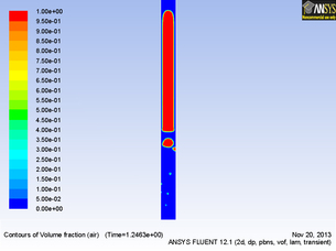
Why model volcanic activity? The benefits and problems #Volcanoes #Modelling #Ansys

Rising Taylor bubble in a vertical tube simulated using Ansys

The fantastic thing about modelling volcanic activity is that we can take our current understanding of the physics surrounding a volcanic problem and apply it safely at a desk. It may not be as exciting as being 'out in the field' but is certainly as valuable as we always need real world data to validate and verify models! Modelling activity takes many forms from investigating the dispersal of ash in the atmosphere for aviation, certainly a very prominent and current problem, to analysing potential lava flow paths, vital for determining potential construction sites. The other arguably most valuable thing about modelling is that it often enables us to see things that we otherwise wouldn't be able to view. For example sub-surface processes such as the motion of magma and gas beneath the surface, which just happens to be my modelling area.

When involved with computational modelling, we try to constantly balance between levels of accuracy, an appropriate representation of the physics involved, computational power, solution time and storage space.

• Accuracy - when running a model you first have to define your area (or geometry), in my case its usually just a simple elongated rectangle. Great! I hear you say. Then we have to mesh the domain, that is define a grid which snaps onto our defined geometry. This is where it starts to get more complex, what kind of mesh do we use, do we make it adaptive (i.e. alters during model run), and the key thing what resolution do we use - too small and solution time may take an eon (and also produce unmanageable amounts of data), too large and we may not be able to represent the physics of the problem sufficiently!
• Appropriate representation of the physics - what equations are we going to use? Are they appropriate for the situation? How long do they take to solve?  
• Computational Power - I can guarantee that this is often the major problem for modellers. I am lucky, in that I have access to the University of Sheffield supercomputer Iceberg (don't ask me why its called that but it sounds cool!) to run applications off and hence a large amount of RAM to draw off. During my MSc I was on the other end of the spectrum, using a desktop computer with 2GB of RAM, waiting 3/4 days to perform 30 s of a model run (probably an under-exaggeration actually). From this you can certainly start to see the challenges mounting up!
• Solution Time - As mentioned above, solution time is certainly key, some climate models can take months to run, which if you are doing a 3 year PhD doesn't leave much room for error! It is therefore inherently important to plan model runs for available time and with available resources.
• Storage Space - In a world where data is easy to create but costly to store this is another key issue. Some of my recent model runs have produced >20 GB of data for just 10 s of model run (and took over 10 hours), when preforming multiple model runs it is obvious that cumulative data production will get larger and quickly run into the terabytes. Some ways of getting around this include only exporting/saving the data you actually need, if your only interested in temperature outputs only save this!

There are many excellent fluid dynamics software applications in existence, however, they are usually costly (running into the tens of thousands, notable exception here is OpenFoam). It is lucky therefore that the University of Sheffield has access to one of the leading applications Ansys and the dynamic Ansys Fluent package. Below is an example of Ansys Fluent model run, simulating the rise of a volcanic slug, generally believed to be the cause of strombolian eruptions at the such volcanoes as the archetypal Stromboli. Cheaper applications such as Matlab, certainly offer the ability to perform, less complex physics problems but lack the user-friendly interfaces such as Ansys and necessitate an in-depth knowledge of the maths and physics behind the problem!

I am sure I have missed many considerations off here, but these are just a few tasters!

It is vitally important that models are not just used on their own, as there is nothing to calibrate or validate the model against. The best way of modelling is by comparing observations in the field, in my case gas emissions, with laboratory proxies, and models. Anyhow, when weighing all of these points against the benefits, a clear and greater understanding of environmental processes is essential and is something which can only occur with significant modelling of processes.

Below is an example simulation of a taylor bubble (or slug) rising through a tube as a proxy for the root cause of a strombolian eruption (the type seen at stromboli).

---